the landscape function

Now we have described our simm adequately, we can start to put it to use. In this post, a brief one, the landscape function. I guess briefly, the landscape function maps an incoming pattern f into a mathematical surface, though almost always that surface is not continuous/smooth.

Say we have a different pattern g(x) at each point x, then simply enough:
L(f,x) = simm(f,g(x))

So, what use is this? To be honest I haven't used it much, but perhaps something like this. Say you have mapped an image of your lounge-room into superpositions of features at point x in the room. ie, we have a g(x). This of course is currently hard!

At x0 we might have g(x0) = |object: light switch>
At x1 we might have g(x1) = |object: books> + |object: book-shelf>
At x2 we might have g(x2) = |object: TV>
and so on.

Then consider say f = |object: TV>, then:
x such that L(f,x) > 0 gives the set of points in the image that contain a TV.

If f = |object: light switch>, then:
x such that L(f,x) > 0 gives the set of points in the image that contain a light switch.
and so on.

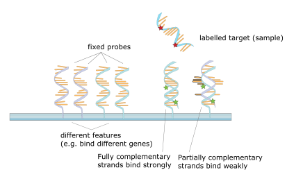
Another perhaps better example is consider DNA microarrays. Here is a picture borrowed from wikipedia:

So in this case, g(x) can be considered to be the DNA pattern at location x.
And f is the target sample of DNA. So, a nice physical implementation of the landscape function. And I guess we are indirectly implying the strength of bonding between DNA strands has a strong similarity with the simm. Something we can realise if we find a good mapping between a DNA sequence and a superposition. Hrmm... maybe we need sequences instead! Anyway, DNA vs BKO is something that calls for more thought.

I guess that is about it for this post.

Home
previous: a superposition implementation of simm
next: introducing similar op x

updated: 19/12/2016
by Garry Morrison
email: garry -at- semantic-db.org