image histogram similarity

In this post I'm going to briefly look into image histogram similarity. Recall our pattern recognition claim:

"we can make a lot of progress in pattern recognition if we can find mappings from objects to well-behaved, deterministic, distinctive superpositions"

where:
1) well-behaved means similar objects return similar superpositions
2) deterministic means if you feed in the same object, you get essentially the same superposition (though there is a little lee-way in that it doesn't have to be 100% identical on each run, but close)
3) distinctive means different object types have easily distinguishable superpositions.

and the exact details of the superposition are irrelevant. Our simm will work just fine. We only need to satisfy (1), (2) and (3) and we are done!

So, today I discovered a very cheap one for images, that has some nice, though not perfect, properties. Simply map an image to a histogram. The Pillow image processing library makes this only a couple of lines of code:

from PIL import Image
im = Image.open("Lenna.png")
result = im.histogram()

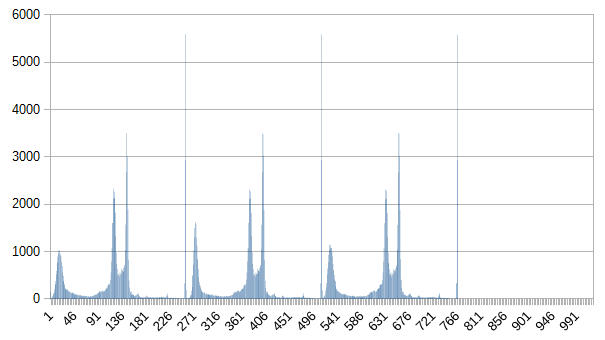
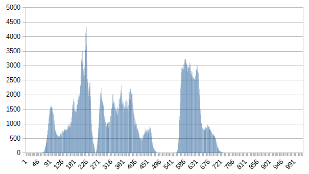
Here are some resulting histograms:
Lenna.png:

small-lenna.png (note that it has roughly the same shape as Lenna.png, but smaller amplitude):

child.png:

three-wolfmoon-output.png:

Now let's throw them at simm. Noting first that we have a function-operator wrapper around im.histogram() "image-histogram[image.png]" that returns a superposition representation of the histogram list:

sa: the |Lenna sp> => image-histogram[Lenna.png] |>
sa: the |small Lenna sp> => image-histogram[small-lenna.png] |>
sa: the |child sp> => image-histogram[child.png] |>
sa: the |wolfmoon sp> => image-histogram[three-wolfmoon-output.png] |>
sa: table[sp,coeff] 100 self-similar[the] |Lenna sp>
+----------------+--------+
| sp             | coeff  |
+----------------+--------+
| Lenna sp       | 100.0  |
| small Lenna sp | 74.949 |
| child sp       | 50.123 |
| wolfmoon sp    | 30.581 |
+----------------+--------+

sa: table[sp,coeff] 100 self-similar[the] |child sp>
+----------------+--------+
| sp             | coeff  |
+----------------+--------+
| child sp       | 100    |
| small Lenna sp | 71.036 |
| Lenna sp       | 50.123 |
| wolfmoon sp    | 44.067 |
+----------------+--------+

sa: table[sp,coeff] 100 self-similar[the] |wolfmoon sp>
+----------------+--------+
| sp             | coeff  |
+----------------+--------+
| wolfmoon sp    | 100.0  |
| child sp       | 44.067 |
| small Lenna sp | 43.561 |
| Lenna sp       | 30.581 |
+----------------+--------+

So it all works quite well, and for essentially zero work! And it should be reasonably behaved with respect to rotating, shrinking (since only the shape of superpositions and not the amplitude matters to simm), adding some noise, removing part of the image, and adding in small sub-images. Note however that it is a long, long way from a general purpose image classifier (I'm confident that will require several layers of processing, here we are doing only one), but is good for very cheap image similarity detection. eg, it would probably easily classify scenes in a movie that are similar, but with a few objects/people/perspective changed.

Now, how would we do the more interesting general purpose image classifier? I of course don't know yet, but I suspect we can get someway towards that using what I call image-ngrams, and our average-categorize code. An image-ngram is named after letter/word ngrams, but is usually called an image partition. The analogy is that just like letter-ngrams[3] splits "ABCDEFG" into "ABC" + "BCD" + "CDE" + "DEF" + "EFG", image-ngrams[3] will partition an image into 3*3 squares. Another interpretation is that letter-ngrams are 1D ngrams, while image-ngrams are 2D. The plan is to then map those small images to a superposition representation, and apply average-categorize to those. With any luck the first layer of average-categorize will self tune to detect edge directions. ie, horizontal lines, or 45 degree lines and so on. It may not work so easily, but I plan to test it soon.

Hrmm... perhaps we could roughly measure how good our object to superposition mappings are, by the number of invariances they have. The more the better the mapping. The image to histogram mapping already has quite a few! On top of those I mentioned above, there are others. You could cut an image horizontally in half, and swap the top for the bottom and you would get a 100% match. Indeed, any shuffling of pixel locations, but not values, will also give a 100% match.

Home
previous: towards a definition of intelligence
next: new tool edge enhance

updated: 19/12/2016
by Garry Morrison
email: garry -at- semantic-db.org